
Orthogonal Array Testing in Practice

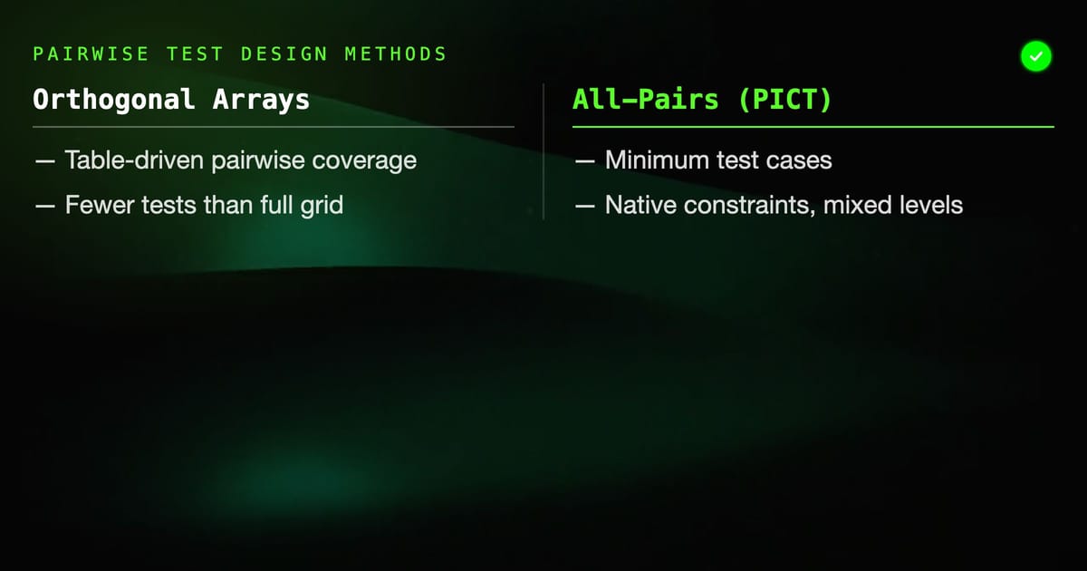
Orthogonal array testing is one of those techniques that gets mentioned in ISTQB study materials and promptly forgotten because the explanation is usually too abstract to be actionable. It shouldn't be. Orthogonal arrays are a concrete, table-driven approach to combinatorial test design with a clean mathematical basis and genuine practical value. Once you understand the structure, applying them is fast and tool-assisted.
This post explains what orthogonal arrays are, where they came from, how they apply to software testing, what L9 and L16 mean, when to prefer orthogonal arrays over all-pairs, and a worked example you can follow.
Origins: Taguchi and Industrial Quality Control
Orthogonal arrays entered software testing via industrial engineering, specifically the work of Genichi Taguchi at Nippon Telephone and Telegraph in the 1950s and 60s. Taguchi was working on the problem of product quality optimization — how to design experiments that efficiently identify which manufacturing parameters most affect product quality, without running every possible combination of settings.
His answer was a set of pre-designed experimental plans called orthogonal arrays (OAs), built on principles from combinatorial design theory. The key property: each array is designed so that for any pair of columns (factors), every combination of factor levels appears the same number of times. This balanced distribution ensures that the effect of any factor can be estimated independently of the effects of other factors.
Taguchi applied this to reduce the number of experiments needed to optimize manufacturing processes by orders of magnitude. The same principle applies directly to software configuration and integration testing.
The technique was introduced to software testing by Kaner, Falk, and Nguyen in "Testing Computer Software" and later formalized by Mandl, who applied orthogonal Latin squares to test design. It predates modern all-pairs algorithms but shares the same underlying goal.
What Makes an Array Orthogonal?
An orthogonal array OA(N, k, v, t) has four parameters:
- N: Number of rows (test cases)
- k: Number of columns (parameters/factors)
- v: Number of levels (values per parameter — assumes all parameters have the same number of values)
- t: Strength (interaction coverage level; t=2 means all pairs covered)
The defining property: in any t columns of the array, every combination of t values appears exactly N/v^t times. Not "at least once" — exactly the same number of times. This balanced coverage is orthogonality.
For t=2 (pairwise), every pair of column values appears the same number of times across all test cases. This is a stronger statement than all-pairs coverage (which requires "at least once") — orthogonal arrays are balanced, not just covering.
The practical difference is minor for defect detection purposes, but the mathematical structure makes orthogonal arrays easier to reason about and precompute. The Taguchi arrays (L4, L8, L9, L12, L16, L18, L27, etc.) are precomputed for specific parameter counts and value counts. You look up the right array for your scenario rather than running an algorithm.
The Standard Taguchi Arrays
Taguchi arrays are named by the number of rows: L4, L8, L9, L12, L16, L18, L27.
L4 Array
Handles: 3 parameters, 2 levels each (binary parameters), 4 test cases
| Test | P1 | P2 | P3 |
|---|---|---|---|
| 1 | 1 | 1 | 1 |
| 2 | 1 | 2 | 2 |
| 3 | 2 | 1 | 2 |
| 4 | 2 | 2 | 1 |
Any two columns contain all four combinations (1,1), (1,2), (2,1), (2,2) exactly once each. Fully balanced.
L4 is the minimum orthogonal array for testing three binary factors with pairwise coverage. Full coverage of 3 binary parameters needs 8 tests. L4 does it in 4.
L9 Array
Handles: 4 parameters, 3 levels each, 9 test cases
| Test | P1 | P2 | P3 | P4 |
|---|---|---|---|---|
| 1 | 1 | 1 | 1 | 1 |
| 2 | 1 | 2 | 2 | 2 |
| 3 | 1 | 3 | 3 | 3 |
| 4 | 2 | 1 | 2 | 3 |
| 5 | 2 | 2 | 3 | 1 |
| 6 | 2 | 3 | 1 | 2 |
| 7 | 3 | 1 | 3 | 2 |
| 8 | 3 | 2 | 1 | 3 |
| 9 | 3 | 3 | 2 | 1 |
Check any two columns: every combination of (1,2,3)×(1,2,3) appears exactly once. 9 test cases from a possible 81 (3^4). Full pairwise balance achieved.
L9 is one of the most useful arrays in software testing — four 3-valued parameters is a common scenario.
L16 Array
Handles: 15 parameters, 2 levels each, 16 test cases (or subsets of these columns)
L16 is a 16×15 array of 1s and 2s. Any two columns contain all four combinations of (2×2) exactly four times each. For binary parameters, this means you can test up to 15 factors with only 16 test cases while maintaining pairwise coverage.
This is powerful for feature flag testing. 15 binary feature flags, fully tested pairwise, in 16 test cases.
L18 Array
Handles: 1 parameter with 2 levels + 7 parameters with 3 levels, 18 test cases
L18 is a mixed-level array — an important category because real systems rarely have all parameters at the same number of values. Mixed-level arrays handle these unequal cases.
The Mixed-Level Problem
Pure orthogonal arrays (like L4, L9, L16) require all parameters to have the same number of levels. Real parameter spaces rarely cooperate. When parameter A has 2 values, B has 3, and C has 4, you can't directly use a standard Taguchi array.
Solutions:
- Use a mixed-level OA (like L18 or L36) that handles different level counts
- Round up to the next power — pad a 2-level parameter to 3 levels by duplicating one value. The array handles 3 levels; the extra rows are still valid test cases.
- Use a modern all-pairs tool (PICT) which handles mixed levels natively without the padding complexity
In practice, most software test scenarios involve mixed level counts, which is why PICT's algorithm — which handles mixed levels directly — is more commonly used than looking up Taguchi tables. Orthogonal arrays are most practical when all parameters have the same number of values, which is less common in software than in manufacturing.
OAT vs All-Pairs: When to Choose Each
Both approaches achieve pairwise coverage. The differences are practical:
| Dimension | Orthogonal Array Testing | All-Pairs (PICT) |
|---|---|---|
| Test case count | Fixed by array structure | Minimum possible |
| Balance | Exactly balanced (each pair same frequency) | At least once (unbalanced) |
| Mixed levels | Awkward, requires padding | Native support |
| Constraints | Not supported natively | Full constraint syntax |
| Tool requirement | Just a lookup table | Needs PICT or equivalent |
| Transparency | Easy to explain and verify | Algorithm output, less transparent |
| Audit trail | Simple table, anyone can verify | Requires tool to reproduce |
Choose OAT when:
- All parameters have the same number of values (or can be padded without distortion)
- You need the test suite to be transparently verifiable (regulatory context, audit)
- You want a fixed, stable test set that doesn't change between runs
- Team members are more comfortable with a lookup table than a tool
- No constraints are needed (or constraints are minimal and can be handled by manual exclusion)
Choose all-pairs (PICT) when:
- Parameters have different numbers of values
- You have constraints to model (invalid combinations)
- You want the minimum possible test suite size
- You're integrating test generation into an automated pipeline
- You need 3-way or higher coverage
For most modern software testing, PICT wins on flexibility. OAT wins on transparency and simplicity for the specific case where the array structure fits.
Worked Example: Web API Configuration Testing
Let's apply L9 to a concrete scenario.
System: A REST API with four configuration parameters, each with 3 values:
- Auth method: API Key, OAuth 2.0, JWT
- Rate limit tier: Free (100 req/hr), Standard (1000 req/hr), Premium (unlimited)
- Response format: JSON, XML, Protobuf
- Cache policy: No cache, 60-second TTL, 24-hour TTL
Full coverage: 3^4 = 81 test cases.
L9 provides pairwise coverage in 9 test cases. Map the 1/2/3 values to actual values:
| Test | Auth Method | Rate Limit | Response Format | Cache Policy |
|---|---|---|---|---|
| 1 | API Key | Free | JSON | No cache |
| 2 | API Key | Standard | XML | 60s TTL |
| 3 | API Key | Premium | Protobuf | 24h TTL |
| 4 | OAuth 2.0 | Free | XML | 24h TTL |
| 5 | OAuth 2.0 | Standard | Protobuf | No cache |
| 6 | OAuth 2.0 | Premium | JSON | 60s TTL |
| 7 | JWT | Free | Protobuf | 60s TTL |
| 8 | JWT | Standard | JSON | 24h TTL |
| 9 | JWT | Premium | XML | No cache |
Verify: pick any two columns, e.g., Auth Method and Cache Policy:
- (API Key, No cache) — Test 1 ✓
- (API Key, 60s TTL) — Test 2 ✓
- (API Key, 24h TTL) — Test 3 ✓
- (OAuth 2.0, 24h TTL) — Test 4 ✓
- (OAuth 2.0, No cache) — Test 5 ✓
- (OAuth 2.0, 60s TTL) — Test 6 ✓
- (JWT, 60s TTL) — Test 7 ✓
- (JWT, 24h TTL) — Test 8 ✓
- (JWT, No cache) — Test 9 ✓
All 9 pairs of (Auth Method, Cache Policy) values are covered, each exactly once. Same verification holds for any other pair of columns.
From 81 combinations to 9, with mathematical pairwise coverage. Each test maps directly to an API call with the specified configuration parameters.
Worked Example: Form Input Testing
Orthogonal arrays also apply to functional input testing, not just configuration. Consider a complex form with four input fields, each with three equivalence classes:
- Name field: Valid name, Empty (error), Special characters (boundary)
- Email field: Valid email, Invalid format (error), Already registered (conflict)
- Password field: Strong (8+ chars, mixed), Weak (too short), Empty (error)
- Country: Valid country code, Invalid code (error), Restricted country (business rule)
Full coverage: 81 combinations. L9 reduces to 9, covering every pair of input conditions:
| Test | Name | Password | Country | |
|---|---|---|---|---|
| 1 | Valid | Valid | Strong | Valid |
| 2 | Valid | Invalid format | Weak | Invalid code |
| 3 | Valid | Already registered | Empty | Restricted |
| 4 | Empty | Valid | Weak | Restricted |
| 5 | Empty | Invalid format | Empty | Valid |
| 6 | Empty | Already registered | Strong | Invalid code |
| 7 | Special chars | Valid | Empty | Invalid code |
| 8 | Special chars | Invalid format | Strong | Restricted |
| 9 | Special chars | Already registered | Weak | Valid |
Every combination of (Name state, Email state) is covered — including (Empty, Already registered) in Test 6, which might trigger interesting server-side behavior when the system tries to look up a registration for an empty string. These edge case interactions are exactly what pairwise testing is designed to expose.
Deriving OAs From Scratch (When Standard Arrays Don't Fit)
When no standard Taguchi array fits your parameter space, you have two options:
Option 1: Use PICT (the practical choice). PICT handles arbitrary parameter counts and level counts without requiring a matching standard array.
Option 2: Construct a mixed OA using Latin squares. This is worth understanding conceptually.
A Latin square is an N×N grid filled with N different symbols such that each symbol appears exactly once in each row and column. This is the building block of orthogonal arrays. An L9 array is essentially constructed from two mutually orthogonal Latin squares of order 3 (MOLS).
The construction process:
- Start with an identity Latin square of order v (the number of levels)
- Find mutually orthogonal Latin squares (MOLS) of the same order
- Stack them as columns to form the OA
The number of MOLS of order v determines the maximum number of parameters in the array. For v=2 (binary), you can have up to v-1=1 orthogonal companion, giving L4 with 3 columns. For v=3, you can have 2 MOLS, giving L9 with 4 columns.
This becomes relevant when you need a custom array for a specific combination that doesn't match standard Taguchi tables. But for practical work, use PICT.
Implementing OAT in a Test Plan
When writing a test plan that uses OAT, document it clearly enough that someone else can reproduce and verify it:
1. List all factors and levels explicitly.
State that you're using an L9 (or L16, etc.) array. Name the reason: "We have 4 factors with 3 levels each; L9 provides all-pairs coverage in 9 test cases compared to 81 for full coverage."
2. Show the mapping explicitly.
Don't just reference the abstract array — show the actual test case table with real values substituted for the 1/2/3 level numbers.
3. Document which pairs are covered.
For review purposes, it's useful to note: "All 6 parameter pairs × 9 value combinations = 54 pairs covered, each appearing exactly once in the 9-test suite."
4. Note what's not covered.
OAT guarantees pairwise coverage but not three-way. If there are known critical three-way interactions, document them separately and add explicit test cases.
5. Add seeds for boundary cases.
The L9 array is the systematic core of the test suite. Supplement it with manually selected cases that are outside the matrix but known to be high-risk. These are seeds in PICT terminology, but in OAT they're just additional rows appended to the table.
Orthogonal Arrays in Regulatory Contexts
In regulated industries, OAT's transparency is a genuine advantage. A reviewer can look at the L9 table and verify — without running any tool — that every pair of factor levels appears exactly once. The proof is in the table structure, not in the algorithm.
For FDA software submissions, DO-178C avionics certification, or IEC 62304 medical device testing, you sometimes need to demonstrate that your test selection method is systematic and documented. A Taguchi array from a standard reference (ISO 11838, the Taguchi reference tables) provides this. The method is citable, the array is fixed, the coverage is verifiable.
PICT output is equally valid for this purpose if you document the tool version and model file, but the transparency argument for OAT is real.
Summary
Orthogonal array testing is a structured, table-based approach to pairwise test design with manufacturing engineering roots. The key arrays — L4, L8, L9, L12, L16, L18, L27 — are pre-built tables you look up rather than generate. Each array provides balanced pairwise coverage: every combination of any two factor levels appears the same number of times.
OAT's strength is transparency and stability: the test suite is a fixed table that anyone can verify without tools. Its weakness is inflexibility with mixed level counts and lack of constraint support, which is why PICT handles most modern software testing scenarios better.
The practical workflow: reach for OAT when parameters are uniform (same number of values each), no constraints are needed, and you want a transparently verifiable test suite. Use PICT for everything else.
Either way, you're replacing random sampling with mathematical structure. That's the point. HelpMeTest can run these parameterized test suites automatically in the cloud without requiring you to manage infrastructure — useful when you have a 16-row or 27-row matrix to execute across environments.